MODELING TREE CONTRIBUTION IN SUSCEPTIBILITY ANALYSIS OF SHALLOW LANDSLIDES
Roberto J. Marín¹ & Juan Pablo Osorio²
Article published in Revista EIA, ISSN 1794-1237 / Year XIV / Volume 14 / Edition N.28 / July-December 2017 / pp. 13-28. DOI: https://doi.org/10.24050/reia.v14i28.975
¹ Civil Engineer. GeoResearch International – GeoR, Environmental School, Faculty of Engineering, University of Antioquia – UdeA. ² Civil Engineer, PGDip, MBA, MEng, PhD, MIEI. GeoResearch International – GeoR, Environmental School, Faculty of Engineering, University of Antioquia – UdeA.
ABSTRACT
In this paper, an assessment of shallow landslide susceptibility in a tropical and mountainous terrain is made. A method that allows modeling slope stability over large areas is used. Tree contribution is quantified by means of three parameters: rainfall interception, root reinforcement, and tree surcharge. A rainfall interception model is used to determine the rain available for infiltration and its temporal distribution during the simulation. The hydrological models included in TRIGRS are described, which allows determining the pore water pressure depending on the initial conditions. This pore water pressure is used in the revised infinite slope stability model, along with root reinforcement and tree surcharge, to determine the slope stability in terms of a factor of safety (FS) for an entire basin. Different scenarios of tree density are modeled in a basin of the Valle de Aburrá, and the results are compared with a model performed without considering the effects of trees on stability.
The results obtained showed values of (FS < 1) (predicting failure with the occurrence of the simulated rainfall event) in a delimited area due to the null presence of trees. On October 26, 2016, months after the investigation was concluded and the paper submitted to Revista EIA, a shallow landslide occurred in the studied area (municipality of Copacabana, landslide on the Medellín-Bogotá Highway K12+200, in the El Cabuyal zone), indicating that the proposed methodology can be a useful tool for the prediction of shallow landslides.
Shallow landslides are an instability phenomenon that primarily affects shallow surficial deposits, generally less than 2 m thick. These are triggered by high-intensity and/or long-duration rainfall events (Montrasio, Schilirò, and Terrone, 2015). Although they mobilize small volumes of soil, they can be abundantly distributed across large territories, often causing damage to crops, structures, and even the loss of human lives (Bordoni et al., 2015a; Bordoni et al., 2015b).
There are various physical models that can analyze the spatial and temporal distribution of shallow landslides at a watershed scale, but the success of these models depends on an appropriate simulation of the terrain characteristics and the mechanisms that trigger this phenomenon (Cascini, Cuomo, and Della Sala, 2011). Thus, the spatial and temporal prediction of rainfall-induced shallow landslides is a difficult task; however, different authors have adopted different methods, among which the following stand out (Raia et al., 2013; Salciarini et al., 2006):
Empirical methods (e.g., Godt, Baum, and Chleborad, 2006; Guzzetti et al., 2008).
Statistical methods (e.g., Coe et al., 2004; Crovelli, 2000; Guzzetti et al., 2006).
Physically based methods (e.g., Burton and Bathurst, 1998; Montgomery and Dietrich, 1994; Montrasio, Valentino, and Losi, 2011; Pack, Tarboton, and Goodwin, 1998; Wu and Sidle, 1995).
Combination of the above (e.g., Frattini, Crosta, and Sosio, 2009; Raia et al., 2013).
Among the factors influencing rainfall-triggered shallow landslides, vegetation properties have an important contribution. The effects of vegetation on slope stability can be grouped into two main types of mechanisms: hydrological and mechanical. Hydrologically, vegetation acts by reducing the water available for infiltration and soil moisture through interception, evaporation, and transpiration. On the other hand, it increases infiltration capacity by increasing soil roughness and promoting the generation of desiccation cracks. Mechanically, the anchoring of roots in more stable soil strata can benefit stability, as can lateral anchoring on surfaces susceptible to failure. Similarly, roots can increase the shear strength of the terrain by providing a reinforcing membrane to the soil layer. Conversely, trees constitute a surcharge that increases the normal and parallel force components to the slope, which can be detrimental to stability. Dynamic forces transmitted by the wind through tree trunks can also represent an adverse mechanism for stability (Gray and Sotir, 1996; Morgan and Rickson, 2003; Sidle and Ochiai, 2006; Stokes et al., 2008).
Although the effects of vegetation on slope stability have been widely studied around the world, few watershed-scale or regional approaches have quantitatively evaluated the contribution of trees associated with the susceptibility of mass movement occurrence (Kim et al., 2013). This article proposes a method to evaluate the susceptibility to rainfall-induced shallow landslides over large areas of terrain (at a watershed scale) by quantifying the effect of trees based on three main parameters: rainfall interception, root reinforcement, and surcharge due to tree weight.
2. GENERAL DESCRIPTION OF THE METHOD
The stability analysis in the evaluated basin is represented by the factor of safety (FS). Using the tools available in a geographic information system, the input data are prepared, adjusted, and introduced. These can be variables with unique values throughout the basin or presented in the form of maps representing their spatial variability. Through a cell configuration, pore pressure and factor of safety calculations are obtained for each one.
To incorporate the effects of trees on stability, a method is implemented that couples existing models (interception, hydrological, and geotechnical models). Thus, Liu’s (1997) rainfall interception model is used, which estimates the rain available for infiltration by reducing the amount intercepted and evaporated from the tree canopy. Next, a transient infiltration model is used to calculate the variation of pore pressure during the simulated rainfall event; in this case, the hydrological component of TRIGRS 2.0 (Baum, Savage, and Godt, 2008) was used. Finally, the revised infinite slope stability model proposed by Kim et al. (2013) is used to determine the factor of safety in each cell, quantifying the surcharge and reinforcement provided by tree roots. The implemented models are detailed below.
2.1. Rainfall Interception Model
Liu’s (1997) interception model is based on the use of physical parameters to estimate rainfall interception according to the following equation:
Where (C_m) is the canopy storage capacity, (D_i) is the canopy dryness index before the rain, (D) is the canopy dryness index, (b_0) is the free drainage coefficient, (\bar{e}) is the average evaporation rate of the wet canopy, (\bar{R}) is the average intensity, and (T) is the time period.
In the present study, Equation (1) is applied for each time interval (which is associated with an average precipitation or intensity value) that makes up the rainfall event, obtaining the canopy dryness index of each period according to the equation shown below, starting with a value of (D_i = 1), which assumes a dry canopy before the rainfall event:
Where (k = 1 – b_0) is the soil cover and (P) is the average precipitation in the time period.
2.2. Modeling Shallow Landslides
TRIGRS is software designed to model the spatial and temporal distribution of rainfall-induced shallow landslides. The program calculates pore pressure changes and determines the variability of the factor of safety due to rainfall infiltration (Baum, Savage, and Godt, 2008). This program couples a hydrological model that simulates rainfall infiltration with an infinite slope stability model, which represents the stability of individual cells using the factor of safety. The landslide susceptibility analysis method in this research adopts only the hydrological model of TRIGRS 2.0, while the geotechnical component (i.e., a simulation applying the entire TRIGRS model) is used to compare the obtained results.
2.3. Hydrological Model
The model assumes flow in homogeneous and isotropic soil, and only vertical one-dimensional infiltration is modeled. TRIGRS 2.0 includes models for saturated and unsaturated initial conditions. For saturated conditions, the infiltration models are based on the linear solution of Richards’ equation (1931), proposed by Iverson (2000). This solution is composed of a steady-state component and a transient component. For pore pressure calculation, the program allows a solution for the case of an infinite depth basal boundary and for a finite depth, representing different subsurface conditions. The former applies where hydraulic conditions are uniform at depth, while the latter represents the case where there is a considerable reduction in hydraulic conductivity at a finite depth.
The generalized solution for an infinite depth basal boundary is given by Equation (3):
Where (\psi) is the pore pressure (in pressure head units); (t) is time; with (Z = z/\cos \delta), (Z) being the coordinate in the vertical direction (positive downwards) and the depth below the soil surface, (z) the coordinate in the direction normal to the slope (positive downwards), and (\delta) is the slope angle; (d) is the steady-state depth of the water table measured in the vertical direction.
Likewise, (\beta = \cos^2 \delta – (I_{ZLT}/K_s)), where (K_s) is the saturated hydraulic conductivity in the (Z) direction, (I_{ZLT}) is the steady (initial) infiltration rate at the surface, (I_{nZ}) is the infiltration rate at a given intensity for the (n)-th time interval.
In turn, (D_1 = D_0/\cos^2 \delta), where (D_0) is the saturated hydraulic diffusivity ((D_0 = K_s/S_s), where (S_s) is specific storage); (N) is the total number of intervals. The terms (H(t-t_n)) represent the Heaviside step function, where (t_n) is the time in the (n)-th interval in the rainfall infiltration sequence.
Where (\text{ierfc}(\eta)) is the complementary error function.
On the other hand, the pore pressure solution for the case of an impermeable basal boundary, for a finite depth (d_{LZ}), is illustrated in Equation (5), where the same notation from Equation (3) is adopted and the term (d_{LZ}) is the depth of the impermeable basal boundary, measured in the (Z) direction.
Additionally, the program allows using an analytical solution for unsaturated flow to estimate infiltration. In this condition, the soil is analyzed as a two-layer system, where a saturated zone with a capillary fringe above the water table borders an unsaturated zone that extends to the soil surface. For this, TRIGRS uses a coordinate transformation described by Iverson (2000) of the one-dimensional analytical solution of Richards’ equation (1931), which describes infiltration and vertical flow through the unsaturated zone, as shown below:
With (K(\psi) = K_s \exp(\alpha\psi^)), where (\psi) is the pressure head, with (\psi^ = \psi – \psi_0), (\psi_0) being a constant ((\psi_0 = 0) or (\psi_0 = -1/\alpha)); (K(\psi)) is a hydraulic conductivity function, (K_s) is the saturated hydraulic conductivity; with (\theta = \theta_r + (\theta_s – \theta_r)\exp(\alpha\psi^*)), (\theta) being the volumetric water content, (\theta_r) the residual volumetric water content, (\theta_s) the volumetric water content at saturation, and (\alpha) a parameter obtained by fitting (K(\psi)) to a soil characteristic curve.
2.2.2. Geotechnical Model Used in TRIGRS
TRIGRS models slope stability using a one-dimensional infinite slope stability analysis, according to Taylor (1948). In this analysis, failure in an infinite slope is characterized by the relationship between resisting friction forces and destabilizing forces induced gravitationally. This relationship represents the factor of safety, which is calculated at a depth (Z), as shown below:
Where (c’) is the effective soil cohesion, (\phi’) is the effective friction angle, (\gamma_w) is the unit weight of water, (\gamma_s) is the unit weight of soil, and (\psi(Z,t)) is the pore pressure (in pressure head units). FS is calculated for pore pressures at different soil depths (Z). Failure is predicted when (FS < 1) and stability when (FS \geq 1), with limit equilibrium at (FS = 1). Since TRIGRS allows calculating FS at different depths, the landslide initiation depth is predicted at the minimum depth where FS is less than 1.
In Baum, Savage, and Godt (2008), additional information is available that describes in detail both the hydrological models and the geotechnical model adopted in the program.
2.3. Revised Infinite Slope Stability Model by Kim et al. (2013)
Kim et al. (2013) integrated a hydrological model (Baum, Savage, and Godt, 2002), a rainfall interception model (Rutter et al., 1971; Rutter, Morton, and Robins, 1975), and a modification to an infinite slope stability model (Hammond et al., 1992), which quantifies the contribution of trees to slope stability to analyze the susceptibility of large terrain areas to shallow landslides. The modified FS equation, which includes the terms for root reinforcement and tree surcharge, allows integrating the spatial and temporal changes of pore pressure modeled by TRIGRS, as shown in the following expression:
Where (c_r) is the reinforcement provided by tree roots, (c’) the effective cohesion, (m_t) the tree surcharge, (\gamma_s) the soil unit weight, (Z) the soil depth, (\delta) the terrain angle, (\psi(Z,t)) the pore pressure as a function of time and soil depth, (\gamma_w) the unit weight of water, and (\phi’) the effective friction angle of the soil.
Thus, the proposed method couples Liu’s (1997) rainfall interception model, used to determine the rain available for infiltration to be used in the simulation with one of the TRIGRS 2.0 hydrological models, selected according to initial boundary and saturation conditions. Spatial and temporal pore pressure changes are obtained from the hydrological modeling, and this term is included in the FS equation of the revised infinite slope stability model by Kim et al. (2013), which includes the terms for tree root reinforcement and surcharge. The proposed method is tested by simulating different tree density scenarios over a basin and comparing the results with a modeling performed in TRIGRS 2.0, without including the effects of trees on stability.
3. CASE STUDY
3.1. Study Site
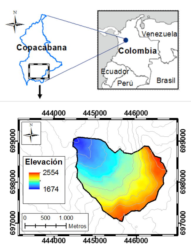
A small basin in the Valle de Aburrá, a subregion of the department of Antioquia (Colombia), is studied. It is located in the El Cabuyal sector, in the municipality of Copacabana. It has an area of 2.94 km² and an elevation range of 1674 m at the basin outlet and 2554 m at the top of the watershed divide. The average precipitation is 1875 mm/year, with relatively constant rainfall. The average temperature is 22.5 °C. The soil types in the El Cabuyal area are classified as alluvial surfaces, mountains, and colluvial soils (ISEA Ltda, 2006).
Figure 2. Location and digital elevation model of the basin.
3.2. Geotechnical and Hydrological Conditions
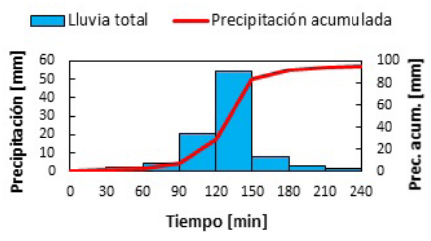
The modeling was performed with a 4-hour design storm. This rainfall event was elaborated from IDF curves defined for the study area (Smith and Vélez, 1997). The hyetograph was constructed using the alternating block method (Chow, Maidment, and Mays, 1988), choosing a return period of 750 years. The resulting rain has an accumulated precipitation of 95.7 mm distributed in 8 intervals of 30 minutes, each with a specific average intensity (Figure 1).
Figure 1. Synthetic hyetograph of the rainfall event to be modeled. It shows precipitation (mm) in 30-minute intervals and accumulated precipitation (mm).
For the simulations, digital terrain maps with a spatial resolution of 10 m x 10 m were generated. Using ArcGIS, a digital elevation model (Figure 2), a flow direction map, and a terrain slope map were created.
Marín and Castro (2015) analyzed shallow landslide susceptibility in this same basin, implementing the TRIGRS 2.0 infiltration model under saturated conditions, adopting a constant soil depth value, and defining the water table height at this same depth. Likewise, they defined the geotechnical ((c’), (\phi’), (\gamma_s)) and hydrological ((K_s), (D_0), (\theta_s), (\theta_r), (I_{ZLT})) variables according to values found in the literature for the soil type found in the area.
Because in many cases there are limitations in obtaining sufficient information on soil conditions, in other modeling with TRIGRS the depth of the sliding surface (assumed as the soil depth or boundary between surficial deposits and bedrock) has been defined as constant (Liao et al., 2011; Montrasio, Valentino, and Losi, 2011; Park, Nikhil, and Lee, 2013; Vieira and Fernandes, 2010), generally with values between 1 m and 2 m, since most shallow landslides occur between these depths (Meisina and Scarabelli, 2007). On the other hand, other authors who have used TRIGRS have chosen to use exponential functions that relate this boundary to the slope angle (Baum, Godt, and Savage, 2010; Salciarini et al., 2006).
The present modeling considers the soil depth with a lower limit of 1.5 m and an upper limit of 1.8 m, implementing the exponential function used by Baum, Godt, and Savage (2010), where the depth of the impermeable basal boundary (d_{LZ}) is a function of the slope angle ((\delta)), (d_{LZ} = 5.0\exp(-0.04\delta)).
Meanwhile, the water table depth prior to the storm has been simulated at the same level (Kim et al., 2013; Kim et al., 2010; Montrasio, Valentino, and Losi, 2011; Park, Nikhil, and Lee, 2013; Vieira and Fernandes, 2010) or as a fraction (Liao et al., 2011; Raia et al., 2013; Salciarini et al., 2006) of the soil depth. In the present study, the initial water table depth ((d)) is simulated as a fraction of this impermeable basal boundary. Thus, (d = 0.75d_{LZ}).
Since at the basin scale it is not easy to have precise information on the spatial variability of soil properties, average values are usually assigned for many of the geotechnical and hydrological parameters in these types of models. In this case, the required variables were defined from information taken from geotechnical studies conducted in this basin, provided by other researchers, and from values taken from the literature for the soil type found in the area. Such field studies consisted of 29 exploratory boreholes in which the water table depth was determined, and through laboratory tests, geotechnical, moisture, and soil strength parameters were obtained. Based on this, an effective cohesion value of 9 kN/m², an effective friction angle of 24°, and a soil unit weight of 15 kN/m³ were assigned, constant throughout the basin. Meanwhile, the simulation of hydrological variables was based on the existing dependence (correlation) between some of these variables (Raia et al., 2013), the aforementioned field and laboratory studies, and a literature search.
In this way, a value of 5.0 x 10⁻⁵ m/s was determined for the saturated hydraulic conductivity ((K_s)). Some authors have established the hydraulic diffusivity term ((D_0)) as a multiple of conductivity (Baum, Godt, and Coe, 2011; Baum, Godt, and Savage, 2010; Bordoni et al., 2015b). Park, Nikhil, and Lee (2013) and Liu and Wu (2008) state that (D_0) is usually between 10 and 500 times the value of (K_s); in both investigations, they adopt a value of (D_0 = 200 K_s). In this research, this relationship is adopted, therefore (D_0 = 1.0 \times 10^{-2}) m²/s. Likewise, both investigations defined the initial infiltration rate as (I_{ZLT} = 0.01 K_s). For this research, this expression is adopted, such that (I_{ZLT} = 5.0 \times 10^{-7}) m/s. Finally, the saturated water content ((\theta_s)) and residual ((\theta_r)) are established with values of 0.45 and 0.1, respectively, and the parameter (\alpha), which approximates the inverse of the capillary fringe height above the water table, is assigned a value of 1 m⁻¹, so the simulation assumes a thick capillary fringe.
The values assigned to each of the required parameters in the modeling of pore pressure and the TRIGRS 2.0 geotechnical model are summarized in Table 1.
TABLE 1. VALUES OF THE GEOTECHNICAL AND HYDROLOGICAL PARAMETERS USED IN THE MODELING
Parameter
Value
(I_{ZLT}) (m/s)
5.0 x 10⁻⁷
(c’) (kN/m²)
9
(\phi’) (°)
24
(\gamma_s) (kN/m³)
15
(K_s) (m/s)
5.0 x 10⁻⁵
(D_0) (m²/s)
1.0 x 10⁻²
(\theta_s)
0.45
(\theta_r)
0.1
(\alpha) (m⁻¹)
1
Similarly, the required variables in the rainfall interception model are defined. Table 2 shows the adopted values for these variables.
TABLE 2. VALUES OF THE RAINFALL INTERCEPTION MODEL VARIABLES
Variable
Value
(b_0)
0.59
(C_m) (mm)
0.78
(\bar{e}) (mm/h)
0.35
(k)
0.41
The reinforcement provided by the roots ((c_r)) and the tree surcharge ((m_t)) were modeled in three different scenarios, for which the values of (c_r) and (m_t) vary according to the simulated tree density case.
TABLE 3. VALUES OF ROOT REINFORCEMENT ((c_r)) AND TREE SURCHARGE ((m_t)) FOR THE MODELED SCENARIOS
Scenario
(c_r) (kN/m²)
(m_t) (kN/m²)
1: Low Tree Density Basin
0.4
0.5
2: High Tree Density Basin
2.0
1.8
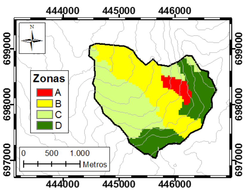
3: Variable Tree Density
Zone A: 0 Zone B: 0.5 Zone C: 0.9 Zone D: 2.0
Zone A: 0 Zone B: 0.4 Zone C: 0.8 Zone D: 1.8
Figure 3. Zones differentiated by tree density in the basin. Zone A: no tree presence ((c_r = 0), (m_t = 0)). Zone B: low tree density ((c_r = 0.5) kN/m², (m_t = 0.4) kN/m²). Zone C: intermediate tree density ((c_r = 0.9) kN/m², (m_t = 0.8) kN/m²). Zone D: high tree density ((c_r = 2.0) kN/m², (m_t = 1.8) kN/m²).
4. RESULTS AND ANALYSIS
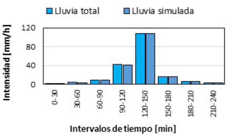
The simulated rainfall, obtained after evaluating the amount intercepted by the tree canopy, is compared with the total rainfall in the hyetographs shown in Figure 4. In this simulation, the total amount of intercepted rain during the entire storm is 2.1 mm, which corresponds to 2.2% of the total precipitation. It is observed that the greatest amount of intercepted water occurs in the first hour of the rainfall event, until the dryness index ((D)) is significantly reduced. Thus, in the first thirty minutes, 24.4% of what is intercepted in the entire rainfall event is intercepted, and in the second time interval (30-60 min), 20.4%.
Figure 4. Hyetographs of total rainfall and simulated rainfall. Average intensity (mm/h) in 30-minute time intervals.
When the initial dryness index approaches zero (for the defined time intervals), i.e., (D_0 \approx 0), the storage capacity has almost reached its maximum capacity, and the contribution of rainfall interception is mainly due to the evaporation effect, given by the average canopy evaporation rate ((\bar{e})). Therefore, rainfall interception is very low in these time intervals.
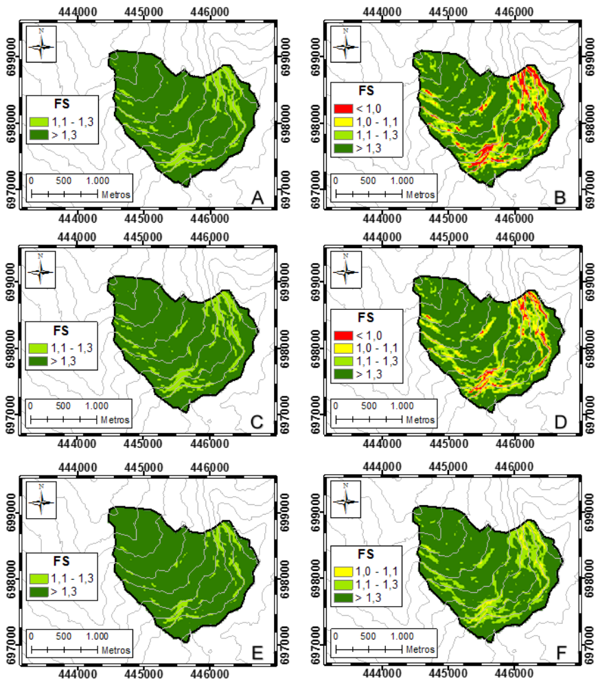
Figures 5 and 6 show the factor of safety (FS) in the four simulations, before and after the duration (4 h) of their design storms. Figures 5a and b show the modeling with TRIGRS 2.0, without considering the effect of trees, from the beginning of the storm ((t = 0), Figure 5a) to its end ((t = 4) h, Figure 5b). Similarly, Figures 5c and d present FS in scenario 1, where a low tree density is simulated throughout the basin ((c_r = 0.4) kN/m², (m_t = 0.5) kN/m²). Likewise, Figures 5e and f show FS in scenario 2, which represents a high tree density throughout the basin ((c_r = 2.0) kN/m², (m_t = 1.8) kN/m²). Finally, Figure 6 shows FS at the beginning and end of the storm for scenario 3, where there is spatial variability of tree density over the basin.
Figure 5. Factor of safety at the beginning (A, C, E) and at the end of the storm (B, D, F). (A – B) Modeling with TRIGRS. (C – D) Scenario 1. (E – F) Scenario 2.
In these simulations, failure is predicted to occur in the cells where FS is less than 1.0. In all modelings, a reduction in FS is observed in multiple cells due to rain water infiltration. Likewise, higher FS values are presented in the scenarios with greater tree density; that is, in those modeled with higher values of (c_r) and (m_t). Thus, in the modeling without considering the arboreal contribution (Figure 5a, b), the lowest FS values were obtained, and the highest number of cells with FS < 1 was presented (failure is predicted in 6.5% of the basin area). Meanwhile, in the scenario where relatively low values of (c_r) and (m_t) are used, simulating low tree density throughout the basin (Figure 5c, d), the cells that fail at the end of the storm decrease by approximately half (3.3% of the basin area with FS < 1), compared to the TRIGRS simulation. In contrast, when simulating a very high tree density throughout the entire basin (Figure 5e, f), the FS values are reduced again at the end of the storm; however, none of the cells fail.
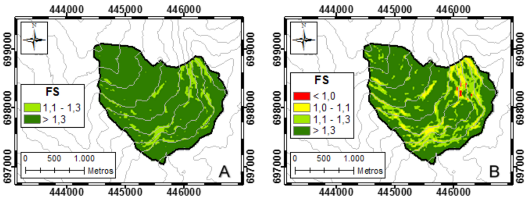
Finally, in the scenario where different zones are delimited according to arboreal presence in differentiated areas of the basin (Figure 6a, b), spatially varying the values of (c_r) and (m_t), few zones presenting instability at the end of the storm are obtained (with 93 cells where FS < 1; i.e., 0.3% of the basin area).
Figure 6. Factor of safety at the beginning (A) and at the end (B) of the storm. Scenario 3, with spatial variability of tree density over the basin. (A) t = 0; (B) t = 4 h.
Comparing the other modelings with the last scenario (Figure 6), where (c_r) and (m_t) vary in the basin according to the tree density of the defined zones, the influence of this delimitation on the obtained results is evident. All the cells where failure is predicted in the simulated tree density scenarios correspond to unstable areas in the modeling performed with TRIGRS. In scenarios 1 and 3, 50.4% and 4.9%, respectively, of the areas that fail in the TRIGRS modeling were predicted. On the other hand, between these scenarios it is observed that, although the unstable area in scenario 3 (variable tree density; Figure 6b) is very small, 44.1% of these are predicted as stable areas in scenario 1 (low tree density; Figure 5d). This is because in some steep slope areas where there is high tree density (scenario 3), there are high (c_r) and (m_t) values that contribute to stability; meanwhile, in most of the terrain where there is very low tree density, the slopes are not steep enough to produce shallow landslides.
The possibility of delimiting small areas within the basin to assign root reinforcement ((c_r)) and surcharge ((m_t)) values according to the observed tree density or other additional information allows simulating the arboreal contribution more precisely than assigning constant values to these variables. The displayed results indicate that the proposed method is very sensitive to the values of (m_t) and (c_r), mainly to the latter. A visual inspection of Equation (8) shows that in the present analysis, (c_r) can be considered as an additional cohesion provided by tree roots. In other investigations, where terms associated with the effect of trees are not included, the cohesion and friction angle values are increased to consider the effect of tree roots in certain areas (e.g., Chien-Yuan et al., 2005). Using TRIGRS tends to overestimate instabilities due to the lack of detailed information on topographic and soil properties throughout the studied area (Jelínek and Wagner, 2007; Kim et al., 2010). Often, the overestimation of landslides in these types of models is because their effects are not quantified in areas with vegetation possessing root systems that contribute to stability (Zizioli et al., 2013).
5. CONCLUSIONS
A method is proposed to analyze the susceptibility to the occurrence of shallow landslides at a watershed scale, including the contribution of trees through three main parameters: rainfall interception, root reinforcement, and surcharge. Liu’s (1997) model is presented as the rainfall interception model that determines the amount of water available for infiltration and its temporal distribution during the event. Likewise, the hydrological models of TRIGRS 2.0 for the simulation of transient infiltration are described according to the types of initial conditions the model allows simulating: saturated and unsaturated, in the types of basal boundaries (finite and infinite) it admits. The pore pressure is calculated with the selected infiltration model and is used in the revised infinite slope stability model by Kim et al. (2013), which includes the terms for root reinforcement and surcharge and represents stability in terms of the factor of safety (FS). FS is calculated for each of the cells that collectively make up the entire basin.
In applying the method in a Valle de Aburrá basin, average values were used for many of the geotechnical and hydrological variables, which actually vary spatially. In basin-scale modeling, these types of simplifications are necessary due to the difficulty of obtaining precise information on their variability throughout the terrain. However, more precise information on these variables would greatly improve the results obtained, which is why many of these types of investigations usually rely on more detailed field information. The same applies to the spatial resolution (10 m x 10 m) of the digital elevation model used. A higher spatial resolution could allow obtaining better results in predicting shallow landslides in these types of simulations (Montrasio, Valentino, and Losi, 2011).
The simulation of different tree density scenarios and the modeling using the TRIGRS model allow observing certain important trends and results. On one hand, a small rainfall interception value (2.1 mm) was obtained in the simulation performed, observing that in the model, interception does not represent a significant component in stability when evaluating high-intensity and short-duration rains. Instead, the reinforcement provided by roots and the tree surcharge have a greater influence on stability, according to the obtained results for the simulated conditions. The possibility of simulating the spatial variability of tree density allows describing real field conditions more adequately and obtaining better results in modeling the contribution of trees to stability.
The proposed method basically presents the same potential disadvantages recognized in the revised model by Kim et al. (2013), as well as other methods that use an infinite slope stability model for predicting shallow landslides. The main one is that these models apply to planar shallow landslides and not to deep mass movements or circular failures. On the other hand, the described method differs in that the employed rainfall interception model uses only physical parameters (no empirical parameters) with specific physical meanings. It also differs in that the TRIGRS 2.0 infiltration models proposed in our method are applicable to a wider range of initial conditions. Although the revised model by Kim et al. (2013) uses the hydrological model of the first version of TRIGRS (Baum, Savage, and Godt, 2002), the TRIGRS 2.0 hydrological model is perfectly applicable to their model.
To study the effects of trees on slope stability more deeply, more investigations of the mechanisms influencing stability are required, as well as conducting modeling under different topographic conditions and rainfall events. The proposed method needs to be applied with more precise variable estimates and a real rainfall event that has caused mass movements on the slopes of a basin, so that actual conditions are simulated as closely as possible and the results can be compared with existing records of the phenomenon.
REFERENCES
Baum, R. L., Savage, W. Z., & Godt, J. W. (2002). TRIGRS–a Fortran program for transient rainfall infiltration and grid–based regional slope–stability analysis (Open-File Report No. 02-424). U.S. Geological Survey. https://doi.org/10.3133/ofr02424
Baum, R. L., Savage, W. Z., & Godt, J. W. (2008). TRIGRS – A Fortran program for transient rainfall infiltration and grid-based regional slope-stability analysis, version 2.0 (Open-File Report No. 2008-1159). U.S. Geological Survey. https://doi.org/10.3133/ofr20081159
Baum, R. L., Godt, J. W., & Savage, W. Z. (2010). Estimating the timing and location of shallow rainfall‐induced landslides using a model for transient, unsaturated infiltration. Journal of Geophysical Research: Earth Surface, 115(F3). https://doi.org/10.1029/2009JF001321
Baum, R. L., Godt, J. W., & Coe, J. A. (2011). Assessing susceptibility and timing of shallow landslide and debris flow initiation in the Oregon Coast Range, USA. In 5th International Conference on Debris-Flow Hazards Mitigation: Mechanics, Prediction, and Assessment (pp. 825–834).
Bordoni, M., Meisina, C., Valentino, R., Bittelli, M., & Chersich, S. (2015a). Site-specific to local-scale shallow landslides triggering zones assessment using TRIGRS. Natural Hazards and Earth System Sciences, 15(5), 1025–1050. https://doi.org/10.5194/nhess-15-1025-2015
Bordoni, M., Meisina, C., Valentino, R., Lu, N., Bittelli, M., & Chersich, S. (2015b). Hydrological factors affecting rainfall-induced shallow landslides: From the field monitoring to a simplified slope stability analysis. Engineering Geology, 193, 19–37. https://doi.org/10.1016/j.enggeo.2015.04.006
Burton, A., & Bathurst, J. C. (1998). Physically based modelling of shallow landslide sediment yield at a catchment scale. Environmental Geology, 35(2-3), 89–99. https://doi.org/10.1007/s002540050296
Cascini, L., Cuomo, S., & Della Sala, M. (2011). Spatial and temporal occurrence of rainfall-induced shallow landslides of flow type: A case of Sarno-Quindici, Italy. Geomorphology, 126(1-2), 148–158. https://doi.org/10.1016/j.geomorph.2010.10.038
Coe, J. A., Michael, J. A., Crovelli, R. A., Savage, W. Z., Laprade, W. T., & Nashem, W. D. (2004). Probabilistic assessment of precipitation-triggered landslides using historical records of landslide occurrence, Seattle, Washington. Environmental & Engineering Geoscience, 10(2), 103–122. https://doi.org/10.2113/10.2.103
Chow, V. T., Maidment, D. R., & Mays, L. W. (1988). Applied hydrology. McGraw-Hill.
Crovelli, R. A. (2000). Probability models for estimation of number and costs of landslides (Open-File Report No. 00-249). U.S. Geological Survey. https://doi.org/10.3133/ofr00249
Frattini, P., Crosta, G., & Sosio, R. (2009). Approaches for defining thresholds and return periods for rainfall-triggered shallow landslides. Hydrological Processes, 23(10), 1444–1460. https://doi.org/10.1002/hyp.7269
Godt, J. W., Baum, R. L., & Chleborad, A. F. (2006). Rainfall characteristics for shallow landsliding in Seattle, Washington, USA. Earth Surface Processes and Landforms, 31(1), 97–110. https://doi.org/10.1002/esp.1237
Gray, D. H., & Sotir, R. B. (1996). Biotechnical and soil bioengineering slope stabilization: A practical guide for erosion control. John Wiley & Sons.
Guzzetti, F., Galli, M., Reichenbach, P., Ardizzone, F., & Cardinali, M. (2006). Landslide hazard assessment in the Collazzone area, Umbria, Central Italy. Natural Hazards and Earth System Sciences, 6(1), 115–131. https://doi.org/10.5194/nhess-6-115-2006
Guzzetti, F., Peruccacci, S., Rossi, M., & Stark, C. P. (2008). The rainfall intensity–duration control of shallow landslides and debris flows: An update. Landslides, 5(1), 3–17. https://doi.org/10.1007/s10346-007-0112-1
Hammond, C., Hall, D., Miller, S., & Swetic, P. (1992). Level I Stability Analysis (LISA) documentation for version 2.0 (General Technical Report INT-285). U.S. Department of Agriculture, Forest Service, Intermountain Research Station. https://doi.org/10.2737/INT-GTR-285
ISEA Ltda. (2006). Plan de saneamiento y manejo de vertimientos – PSMV – Vereda el Cabuyal, municipio de Copacabana-Antioquia.
Iverson, R. M. (2000). Landslide triggering by rain infiltration. Water Resources Research, 36(7), 1897–1910. https://doi.org/10.1029/2000WR900090
Jelínek, R., & Wagner, P. (2007). Landslide hazard zonation by deterministic analysis (Veľká Čausa landslides area, Slovakia). Landslides, 4(4), 339–350. https://doi.org/10.1007/s10346-007-0096-z
Kim, D., Im, S., Lee, S. H., Hong, Y., & Cha, K.-S. (2010). Predicting the rainfall-triggered landslides in a forested mountain region using TRIGRS model. Journal of Mountain Science, 7(1), 83–91. https://doi.org/10.1007/s11629-010-1071-x
Kim, D., Im, S., Lee, C., & Woo, C. (2013). Modeling the contribution of trees to shallow landslide development in a steep, forested watershed. Ecological Engineering, 61, 658–668. https://doi.org/10.1016/j.ecoleng.2013.05.003
Liao, Z., Hong, Y., Kirschbaum, D., Adler, R. F., Gourley, J. J., & Wooten, R. (2011). Evaluation of TRIGRS (transient rainfall infiltration and grid-based regional slope-stability analysis)’s predictive skill for hurricane-triggered landslides: A case study in Macon County, North Carolina. Natural Hazards, 58(1), 325–339. https://doi.org/10.1007/s11069-010-9670-y
Liu, C.-N., & Wu, C.-C. (2008). Mapping susceptibility of rainfall-triggered shallow landslides using a probabilistic approach. Environmental Geology, 55(4), 907–915. https://doi.org/10.1007/s00254-007-1042-x
Marín, R. J., & Castro, J. D. (2015). Efecto de los árboles en la ocurrencia de deslizamientos superficiales en una cuenca del Valle de Aburrá. Universidad de Antioquia.
Meisina, C., & Scarabelli, S. (2007). A comparative analysis of terrain stability models for predicting shallow landslides in colluvial soils. Geomorphology, 87(3), 207–223. https://doi.org/10.1016/j.geomorph.2006.09.016
Montgomery, D. R., & Dietrich, W. E. (1994). A physically based model for the topographic control on shallow landsliding. Water Resources Research, 30(4), 1153–1171. https://doi.org/10.1029/93WR02979
Montrasio, L., Valentino, R., & Losi, G. L. (2011). Towards a real-time susceptibility assessment of rainfall-induced shallow landslides on a regional scale. Natural Hazards and Earth System Sciences, 11(7), 1927–1947. https://doi.org/10.5194/nhess-11-1927-2011
Montrasio, L., Schilirò, L., & Terrone, A. (2015). Physical and numerical modelling of shallow landslides. Landslides, 13(4), 873–883. https://doi.org/10.1007/s10346-015-0642-x
Morgan, R. P. C., & Rickson, R. J. (2003). Slope stabilization and erosion control: A bioengineering approach. Taylor & Francis. https://doi.org/10.4324/9780203011355
Norris, J. E., Greenwood, J. R., Achim, A., Gardiner, B. A., Nicoll, B. C., Cammeraat, E., & Mickovski, S. B. (2008). Hazard assessment of vegetated slopes. In Slope stability and erosion control: Ecotechnological solutions (pp. 119–166). Springer. https://doi.org/10.1007/978-1-4020-6676-4_5
Pack, R. T., Tarboton, D. G., & Goodwin, C. N. (1998). The SINMAP approach to terrain stability mapping. In 8th Congress of the International Association of Engineering Geology (pp. 21–25).
Park, D. W., Nikhil, N. V., & Lee, S. R. (2013). Landslide and debris flow susceptibility zonation using TRIGRS for the 2011 Seoul landslide event. Natural Hazards and Earth System Sciences, 13(11), 2833–2849. https://doi.org/10.5194/nhess-13-2833-2013
Raia, S., Alvioli, M., Rossi, M., Baum, R. L., Godt, J. W., & Guzzetti, F. (2014). Improving predictive power of physically based rainfall-induced shallow landslide models: A probabilistic approach. Geoscientific Model Development, 7(2), 495–514. https://doi.org/10.5194/gmd-7-495-2014
Richards, L. A. (1931). Capillary conduction of liquids through porous mediums. Physics, 1(5), 318–333. https://doi.org/10.1063/1.1745010
Rutter, A. J., Kershaw, K. A., Robins, P. C., & Morton, A. J. (1971). A predictive model of rainfall interception in forests, 1. Derivation of the model from observations in a plantation of Corsican pine. Agricultural Meteorology, 9, 367–384. https://doi.org/10.1016/0002-1571(71)90034-3
Rutter, A. J., Morton, A. J., & Robins, P. C. (1975). A predictive model of rainfall interception in forests. II. Generalization of the model and comparison with observations in some coniferous and hardwood stands. Journal of Applied Ecology, 12(1), 367–380. https://doi.org/10.2307/2401739
Salciarini, D., Godt, J. W., Savage, W. Z., Conversini, P., Baum, R. L., & Michael, J. A. (2006). Modeling regional initiation of rainfall-induced shallow landslides in the eastern Umbria Region of central Italy. Landslides, 3(3), 181–194. https://doi.org/10.1007/s10346-006-0037-0
Sidle, R. C., & Ochiai, H. (2006). Landslides: Processes, prediction, and land use. American Geophysical Union. https://doi.org/10.1029/WM018
Smith, R., & Vélez, M. V. (1997). Hidrología de Antioquia. Secretaría de Obras Públicas Departamentales.
Stokes, A., Norris, J., van Beek, L. P. H., Bogaard, T., Cammeraat, E., Mickovski, S., & Fourcaud, T. (2008). How vegetation reinforces soil on slopes. In Slope stability and erosion control: Ecotechnological solutions (pp. 65–118). Springer. https://doi.org/10.1007/978-1-4020-6676-4_4
Taylor, D. W. (1948). Fundamentals of soil mechanics. John Wiley & Sons.
Vieira, B. C., & Fernandes, N. F. (2010). Shallow landslide prediction in the Serra do Mar, Sao Paulo, Brazil. Natural Hazards and Earth System Sciences, 10(9), 1829–1837. https://doi.org/10.5194/nhess-10-1829-2010
Wu, W., & Sidle, R. C. (1995). A distributed slope stability model for steep forested basins. Water Resources Research, 31(8), 2097–2110. https://doi.org/10.1029/95WR01136
Zizioli, D., Meisina, C., Valentino, R., & Montrasio, L. (2013). Comparison between different approaches to modeling shallow landslide susceptibility: A case history in Oltrepo Pavese, Northern Italy. Natural Hazards and Earth System Sciences, 13(3), 559–573. https://doi.org/10.5194/nhess-13-559-2013